z_norm <- rnorm(1000)
qqnorm(z_norm)
qqline(z_norm)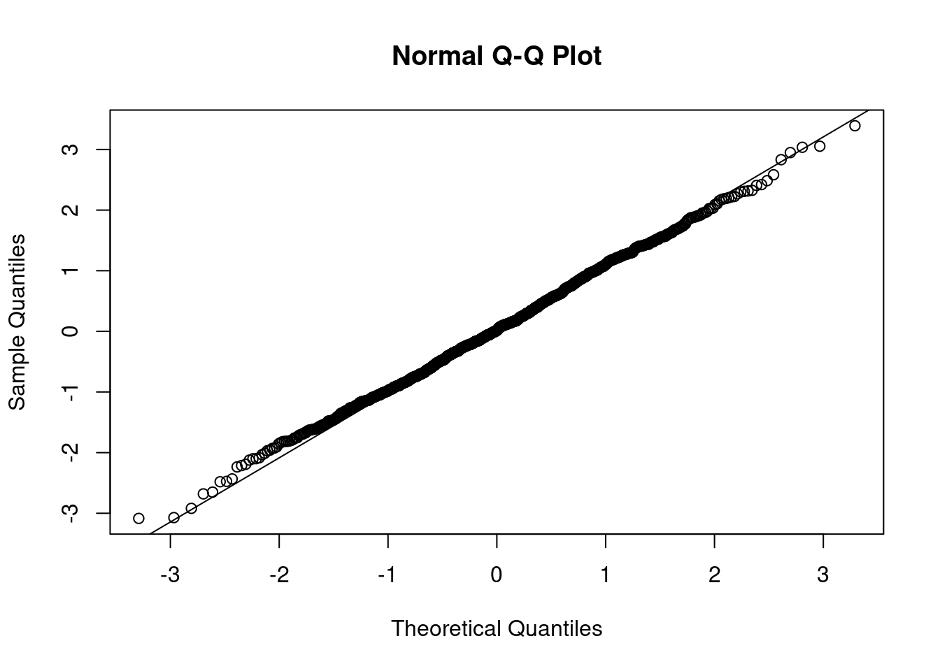
Let \(X_1, X_2, \ldots, X_n\) be identical and independent distributed random variables with \(E(X_i)=\mu\) and \(Var(X_i) = \sigma²\). We define
\[ Y_n = \sqrt n \left(\frac{\bar X-\mu}{\sigma}\right) \mathrm{ where }\ \bar X = \frac{1}{n}\sum^n_{i=1}X_i. \]
Then, the distribution of the function \(Y_n\) converges to a standard normal distribution function as \(n\rightarrow \infty\). The central limit theorem can b reexpressed as:
\[ \bar X \sim N(\mu,\sigma^2/n) \]
To check whether the data follows a normal distribution, we can utilize a QQ-Plot. The main idea is that the points, or quantiles must follow \(f(x)=x\). To create a qq-plot in R, you will use qqnorm(). This will plot the points; additionally, you can use qqline() function to add \(f(x)=x\) to the plot1 The example below will generate 1000 random variables from a standard normal distribution. Then it will create the qq-plot for you to evaluate. You will need to run qqnorm and qqline the same time to get the plot.
z_norm <- rnorm(1000)
qqnorm(z_norm)
qqline(z_norm)
The closer all the points are to the line, the more proof you have that the sample came from a normal distribution.
The normal distribution has 2 finite moments. While the distribution of \(\bar X\) will be normal regardless of sample size, the central limit theorem will still apply.
The code below provides a small simulation study where we will generate nreals random variables from standard normal distribution nsim times. Then we obtain the sample mean for each simulated data set and plot the histogram and QQ-plot.
nsims <- 1000
nreals <- 10000
x <- matrix(nrow = nreals, ncol = nsims)
for(i in 1:nsims){
  x[,i]<- rnorm(nreals)
}
xbar <- colMeans(x)
plot(density(xbar))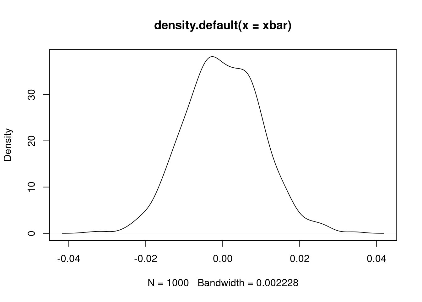
qqnorm(xbar)
qqline(xbar)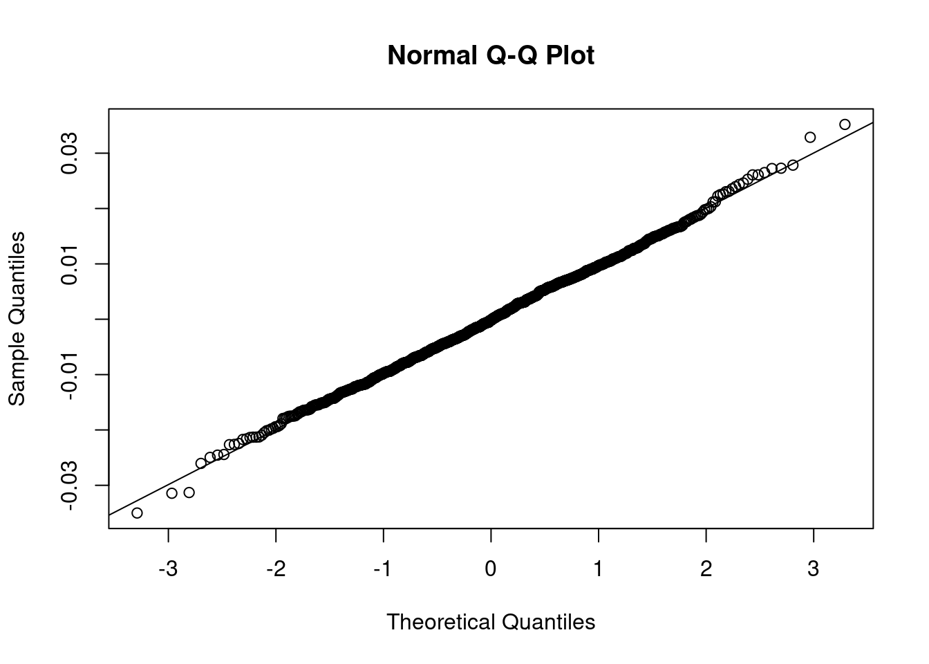
The Cauchy Distribution has and undefined mean and variance; therefore, the central limit theorem does not apply to it.
nsims <- 1000
nreals <- 10000
x <- matrix(nrow = nreals, ncol = nsims)
for(i in 1:nsims){
  x[,i]<- rcauchy(nreals)
}
xbar <- colMeans(x)
plot(density(xbar))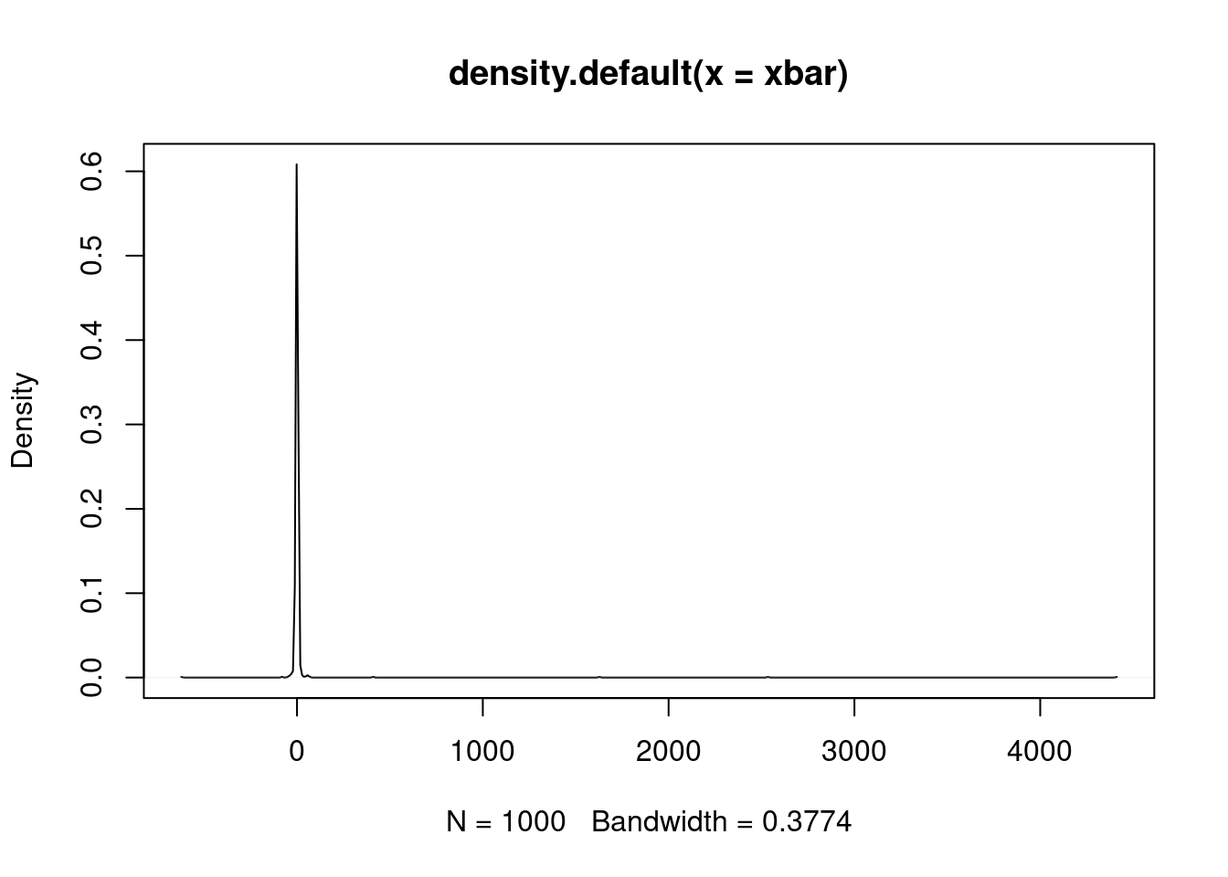
qqnorm(xbar)
qqline(xbar)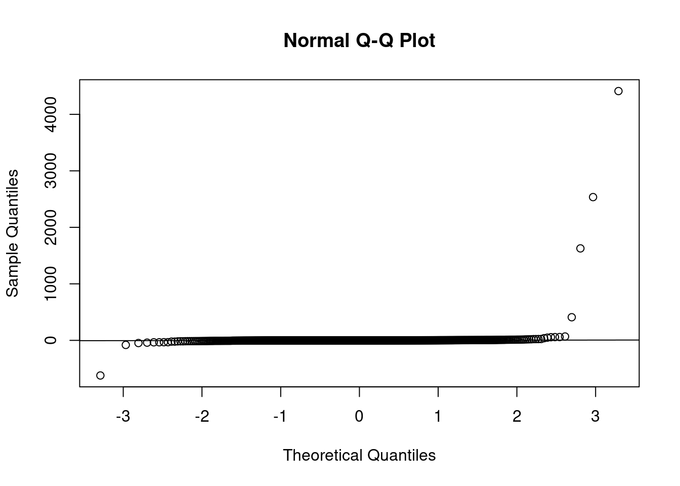
Comment the code below describing the what each line is doing:
nsims <- 1000
nreals <- 10000
x <- matrix(nrow = nreals, ncol = nsims)
for(i in 1:nsims){
  x[,i]<- rnorm(nreals)
}
xbar <- colMeans(x)
plot(density(xbar))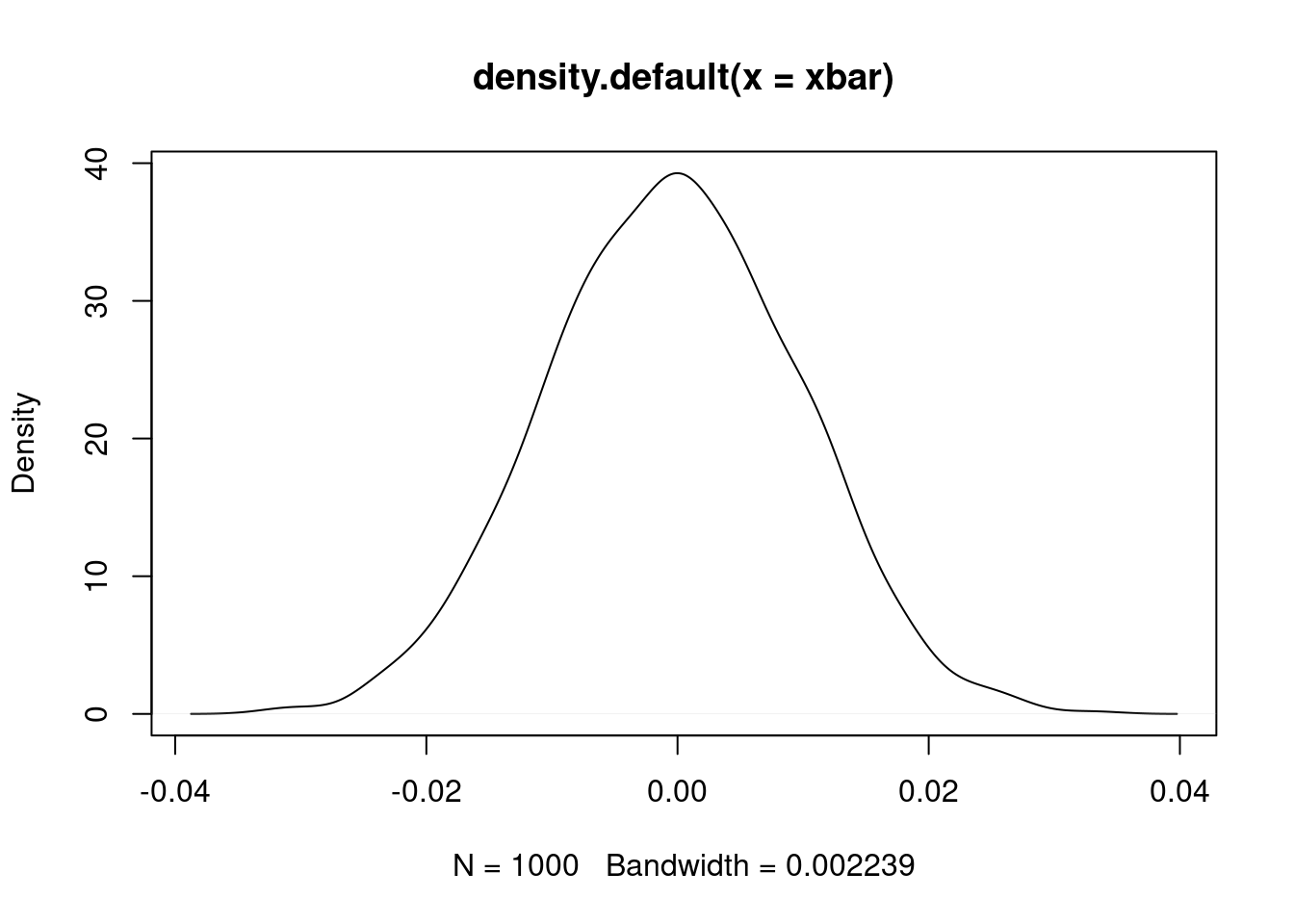
qqnorm(xbar)
qqline(xbar)
Let \(X_1,\ldots, X_n\overset{iid}{\sim}Bernoulli(0.4)\). Does \(\bar X\) follow a normal distribution when the sample size gets larger.
Let \(X_1,\ldots, X_n\overset{iid}{\sim}Gamma(3,4)\). Does \(\bar X\) follow a normal distribution when the sample size gets larger.
Let \(X_1,\ldots, X_n\overset{iid}{\sim}Beta(1,2)\). Does \(\bar X\) follow a normal distribution when the sample size gets larger.
Complete the assignment and submit your code as a QMD file. Submit your file to Canvas on 11/2/2022 at 11:59 PM.
You will need to run both of these lines at the same time.↩︎